(June 2013, Reddit-ed)
Optimizing code for the European Space Agency
Kent Beck

The StrayLight algorithm performs digital processing on data sent from satellites, clearing up unintended lighting effects recorded inside them.
The prototype provided by ESA personnel, was implemented in the IDL programming language. IDL is a near-perfect match for its intended audience, offering an easy way for scientists and engineers to analyze and process data (scalars, vectors, matrices, etc, as well as ready-made library functions for FFTs, interpolations, convolutions, ...)
Moreover, the associated REPL [2] execution environment compiles the IDL code on the fly (in a manner very similar to that of a JIT engine [3]). In collaboration with the highly optimized implementations of the underlying primitives, the end result offered by IDL is an excellent balance between code complexity and run-time speed.
There is, however, room for improvement in that final regard - speed.
The following sections demonstrate how we increased the overall execution speed of the complete StrayLight algorithm (including the PSF computation) in our development machine [4] by a factor of close to 8x, through porting of the IDL code to C++/CUDA. In fact, since the calculation of the PSF data is not frame-dependent [5], the parts of the computation that have to be performed per frame are executing 35 times faster, enabling real-time processing.
1. Output verification
Before optimizing anything, we first had to establish the correctness of our implementation.
To make sure that the results of the C++ implementation would not deviate from the IDL one, logging "stages" were introduced in the original IDL code. These are simply code blocks that can optionally log the contents of 1- or 2-dimensional variables to files, allowing us to perform comparisons of the results.
The original IDL code was thus broken down into 13 stages, each one logging different parts of the computation process's results:
...
; Use debug=1 to enable logging
debug = 0
;debug = 1
...
; Computation of the incidence angle variations in radian
theta0_M1=abs(delta_incidence_angle[0]*!pi/180.*(...
theta0_M2=abs(delta_incidence_angle[1]*!pi/180.*(...
theta0_M3=abs(delta_incidence_angle[2]*!pi/180.*(...

if debug eq 1 then begin
    file_output='./output_data/stage1'
    get_lun, lun_out
    openw, lun_out, file_output
    printf, lun_out, theta0_M1
    printf, lun_out, theta0_M2
    printf, lun_out, theta0_M3
    close, /all
end

...

if debug eq 1 then begin
    file_output='./output_data/stage2'
    get_lun, lun_out

...
The C++ implementation was subsequently built stepwise, verifying that each time a stage was reached, the results did not deviate from the ones generated by IDL. Since the work involved floating point numbers, we begun the implementation with a typedef that would allow easily switching - if necessary - from single to double precision:
$ head src/configStraylight.h
...
typedef float fp;
To be able to compare the output files with configurable degrees of accuracy, we then wrote a simple Python script:
#!/usr/bin/env python
import sys
from itertools import izip

def compare(filename1, filename2):
    elemNo = -1
    lineCnt = 0
    for l1,l2 in izip(open(filename1), open(filename2)):
        lineCnt += 1
        valuesa = l1.split()
        valuesb = l2.split()
        for x,y in zip(valuesa,valuesb):
            if abs(float(x))>1e-10:
                result = abs(float(x)-float(y))/abs(float(x)) > 1e-5
            elif abs(float(y))>1e-10:
                result = abs(float(x)-float(y))/abs(float(y)) > 1e-5
            else:
                elemNo += 1
                continue
            if result:
                print "In line", str(lineCnt)+":", x, y
                print "i.e. element:", elemNo
                sys.exit(1)
            elemNo += 1

if len(sys.argv) != 3:
    print "Usage:" + sys.argv[0] + " <file1> <file2>"
    sys.exit(1)
compare(sys.argv[1], sys.argv[2])
sys.exit(0)
This Python script compares two files, line by line - comparing the contained numbers to a configurable degree of accuracy. The log files it works with are the ones generated by the IDL code - which end up quite big (the algorithm operates on large data buffers). The script therefore doesn't load the file contents in memory all at once, and instead opts to use the iterator protocols of Python - processing each line individually.
Notice that the comparison is not an absolute one: the boolean result is computed based on the relative difference between the two samples, so it adapts nicely to different magnitudes (if both values are too close to zero, it just ignores them).
This comparison process (verifying outputs from all stages) was added as a rule to the Makefile that builds the C++ source code. Every time the C++ code was extended to reach a new stage, a make test was used to verify that the outputs from IDL and C++ did not deviate.
2. Low-hanging fruit
2.1. The matrix types
ESA's prototype IDL code operated on both 1- and 2-dimensional matrices. These were initially represented in the C++ code with:
typedef std::vector<fp>  m1d;
typedef std::vector<m1d> m2d;
- The STL vector type represents data internally by allocating them in a contiguous space on the heap. Cache-performance wise, this means that a vector<fp> is no different than a classic heap-allocated array (fp *pVariable=new Type[...]). The only performance differences to watch for were (a) in the lost low-level optimization opportunities that a plain array offers to a good compiler (inlining, loop-unrolling, etc), as well as (b) the case of 2-dimensional matrices. The effort involved in optimizing these was postponed for later implementation stages.
- The vector<vector<...>> scheme also allowed individual lines of the two dimensional matrix to be assigned to m1d& references, outside the inner-loops. This offered significant speed advantages, as shown below.
2.2. For-loops
By handling vectors and matrices as high-level entities, IDL is in many ways behaving like pure functional languages (e.g. Haskell), which work on immutable data. IDL in fact explicitely states that imperative constructs like for loops impact speed, and counter-suggests using high-level primitives:
theta0_M1 = delta_incidence_angle[0]*!pi/180.*indgen(...
In C++, however, ...
// Computation of the incidence angle variations
m1d  theta0_M1(image_dim_x);
for(i=0; i<image_dim_x; i++) {
    theta0_M1[i] = delta_incidence_angle[0]*M_PI/180.*...
}
...the compiler can utilize low-level speed optimizations inside for loops: it can store variables in registers, thus avoiding memory accesses ; it can unroll the loop, if it figures out that this will be faster. More importantly, it can choose to use SIMD instructions (like Intel SSE or AVX) to significantly speed up the loop (SSE instructions allow operations on 4 floats to be done in one cycle; AVX allows 8).
The run-time library implementation of IDL's base primitives may in fact already be using SIMD instructions; a compiler however, is far better equipped to mix and match various low-level optimizations alongside SIMD implementations - and figure out where using them makes sense and where it doesn't. SIMD-wise, it's the difference between having a technology only in parts of your runtime library, and having it automatically applied wherever in your algorithm it makes sense to do so.
2.3. Mutation of data
Speed-wise, the IDL engine is facing another insurmountable problem: the immutability aspects of many of the operations performed in the original code. For example, this IDL code...
theta0_M1 = delta_incidence_angle[0]*!pi/180.*(indgen(
    image_dim_x)-image_dim_x/2)/...
... describes an operation in terms of actions on immutable vectors. In this case, indgen is utilized to actually generate a vector of size image_dim_x, on whose elements (which are generated to be monotonically increasing) a subtraction of image_dim_x/2 is performed.
Contrast this to the C++ version:
for(i=0; i<image_dim_x; i++) {
    theta0_M1[i] = delta_incidence_angle[0]*M_PI/180.*
        (i-image_dim_x/2)/...
This is far more efficient:
- The C++ version is not wasting memory to create a "temporary" vector. The only reason indgen is used in the IDL code to create this vector (with values from -image_dim_x/2 to image_dim_x/2-1) is that loops are too slow in IDL. C++ has no such problems - and with that factor removed, it is easy to see that indgen is in fact generating a useless vector (from an execution-speed viewpoint).
- More importantly, the extra memory space of the temporary vector "pollutes" the CPU cache. The cache has to handle accesses to this vector's memory just like it does for any other - when in fact, the vector's data will be immediately afterwards thrown out of the cache (with the corresponding penalty of accessing the next required data from the next-level of cache, or even main memory).
The proper utilization of the CPU cache is a common factor in many of the speedups achieved by our C++ code, as we will see in the following sections.
2.4. Memory use and garbage collection
The gdl execution environment (REPL) operates like many other interpreters - it employs garbage collection techniques to perform memory management.
Running top -b allowed us to monitor the memory usage of the execution of both the IDL and the C++ versions of the code:
$ top -b | grep --line-buffered gdl
PID   USER   VIRT  RES  SHR  S %CPU %MEM   TIME+   COMMAND
10288 ttsiod 1282m 1.1g 7988 R   97 18.6   0:04.30 gdl
10288 ttsiod 1282m 1.1g 7988 R  100 18.6   0:07.30 gdl
10288 ttsiod 1282m 1.1g 7988 R  101 18.6   0:07.63 gdl
10288 ttsiod 1134m 819m 7988 R   99 13.7   0:10.63 gdl
10288 ttsiod 1282m 967m 7988 R  100 16.2   0:13.65 gdl
10288 ttsiod 1134m 967m 7992 R  100 16.2   0:16.65 gdl
10288 ttsiod 1430m 1.2g 8004 R   99 21.1   0:17.98 gdl
10288 ttsiod 1430m 1.2g 8004 R  101 21.1   0:20.70 gdl
10288 ttsiod 1430m 1.2g 8004 R  100 21.1   0:22.47 gdl
10288 ttsiod 1430m 1.2g 8004 R   99 21.1   0:25.45 gdl
10288 ttsiod 1578m 1.4g 8004 R  100 23.6   0:28.46 gdl
10288 ttsiod 1578m 1.4g 8004 R  100 23.6   0:29.01 gdl
10288 ttsiod 1578m 1.4g 8004 R  100 23.6   0:32.02 gdl
10288 ttsiod 1874m 1.6g 8004 R  100 27.4   0:35.03 gdl
10288 ttsiod 2171m 2.0g 8004 R  100 33.5   0:38.03 gdl
10288 ttsiod 2171m 2.0g 8004 R  100 33.5   0:41.05 gdl
10288 ttsiod 2171m 2.0g 8004 R  100 33.5   0:44.05 gdl
10288 ttsiod 2171m 2.0g 8004 R  100 33.5   0:47.06 gdl
10288 ttsiod 2171m 2.0g 8004 R  101 33.5   0:47.41 gdl
10288 ttsiod 2319m 2.1g 8004 R  100 35.9   0:50.42 gdl
10288 ttsiod 2171m 2.0g 8004 R  100 33.5   0:53.42 gdl
10288 ttsiod 2911m 2.7g 8004 R  100 45.8   0:56.43 gdl
10288 ttsiod 2911m 2.7g 8004 R  100 45.8   0:59.44 gdl
10288 ttsiod 2911m 2.7g 8004 R  100 45.8   1:02.43 gdl
10288 ttsiod 2911m 2.7g 8004 R  100 45.8   1:05.45 gdl
10288 ttsiod 3059m 2.8g 8004 R  100 48.3   1:08.45 gdl
10288 ttsiod 3059m 2.9g 8004 R  100 48.3   1:11.46 gdl
10288 ttsiod 1282m 1.0g 8024 R  100 17.0   1:14.47 gdl
10288 ttsiod 1282m 1.1g 8024 R  100 18.6   1:17.48 gdl
10288 ttsiod 1282m 1.0g 8024 R  100 17.2   1:20.48 gdl
10288 ttsiod 1430m 1.2g 8024 R  100 21.1   1:23.49 gdl
10288 ttsiod 1430m 1.2g 8024 R  100 21.1   1:26.49 gdl
10288 ttsiod 2023m 1.8g 8024 R  100 31.0   1:29.50 gdl
10288 ttsiod 2023m 1.8g 8024 R  100 31.0   1:32.51 gdl
10288 ttsiod 2171m 1.9g 8024 R  100 32.6   1:35.52 gdl
10288 ttsiod 2171m 2.0g 8024 R  100 33.5   1:38.52 gdl
10288 ttsiod 2023m 1.8g 8024 R  100 31.0   1:41.53 gdl
10288 ttsiod 2763m 2.5g 8024 R  100 43.4   1:44.53 gdl
10288 ttsiod 2763m 2.5g 8024 R  100 43.4   1:47.55 gdl
10288 ttsiod 2911m 2.7g 8024 R  100 45.8   1:50.54 gdl
10288 ttsiod 2911m 2.7g 8024 R  100 45.8   1:53.55 gdl
10288 ttsiod 3059m 2.8g 8024 R  100 48.3   1:56.56 gdl
10288 ttsiod 1295m 1.1g 8044 R  100 18.9   1:59.57 gdl
10288 ttsiod 1759m 1.4g 8768 R  100 24.7   2:02.58 gdl
...

$ top -b | grep --line-buffered strayLight
PID   USER   VIRT  RES   SHR S %CPU %MEM   TIME+   COMMAND
10352 ttsiod 1091m 978m  844 R  123 16.3   0:03.70 strayLight
10352 ttsiod 1245m 1.1g  844 R  593 18.1   0:15.52 strayLight
10352 ttsiod 1102m 1.0g  844 R  551 17.1   0:26.09 strayLight
10352 ttsiod 1318m 1.1g  844 R  570 18.7   0:37.21 strayLight
10352 ttsiod 1242m 1.0g  844 R  573 17.9   0:48.42 strayLight
10352 ttsiod 1089m 972m  864 R  552 16.2   0:59.01 strayLight
10352 ttsiod 1089m 972m  864 R  592 16.2   1:10.78 strayLight
10352 ttsiod 1089m 972m  864 R  597 16.2   1:22.73 strayLight
Focusing on the memory usage columns (VIRT and RES), we observed the following:
- The C++ version of the algorithm used far less memory than the IDL one. As explained in the previous section, this can be attributed to (a) the fact that "temporary" vectors introduced in IDL to avoid for loops are thrown away completely in C++, and (b) in C++ we can modify a vector in-place if it suits our purpose. Both of these factors combine to make C++ use around 1GB of memory, when IDL is using 3GB. This means that CPU caches are stressed a lot more, and inevitably, speed suffers.
- Notice also the pattern of increase: as the algorithm runs, the interpreter is monotonically increasing memory usage, until it reaches 3GB - at which point, a sharp drop is noticed, which brings it down to around 1GB ; and then the cycle repeats. This is very similar to the patterns of other systems where memory is garbage collected - and it has a noticeable impact on speed, which is of course absent from the C++ implementation (where memory is managed explicitely in the matrix classes: allocated in the constructor, released in the destructor).
- Equally important - the absence of a garbage-collection cycle means that the execution profile of the C++ code remains constant: each image is processed in the same time as any other.
Lines in the shell output above were emitted every 3 seconds by top -b; there were a lot more lines while running the IDL code than when running the C++ one, since the overall execution time lasted close to 8 times longer.
The astute reader may be wondering about the results reported in column TIME; but that is easily explained by the fact that this column contains the accumulated time spent in all cores of the machine. The C++ version makes use of all of them (notice the CPU column) - which brings us nicely into discussing the matter of multi-threading.
2.5. Scaling with OpenMP
In the pursuit of execution speed, it is of paramount importance to take advantage of the multiple cores inside modern CPUs.
In the case of IDL, this can only be done in terms of multiprocessing - i.e. running multiple instances of the IDL engine, each one processing a different input image.
This, however, is not as performant as multi-threading from inside a single process. The reason, has to do with the caches' behaviour - and in particular, with their utilization factor:
#ifdef USE_OPENMP
#pragma omp parallel for
#endif
for(int i_y=0; i_y<image_dim_y; i_y++) {
    for(int j=0; j<image_dim_x; j++)
       input_image_corrected[i_y][j] =
            input_image[i_y][j]
            *
            correction_direct_peak[j];
}
This part of our C++ code uses an OpenMP #pragma, directing the compiler to generate code that spawns threads - with each thread processing a different "batch" of i_y scanlines. The key thing to notice here, is that all threads operate on the same buffers: they read from the input_image and correction_direct_peak matrices, and output to input_image_corrected.
In comparison, when multiple instances of this same code are executed concurrently from multiple processes that operate on different images, the Ln cache is, in-effect, completely thrashed. Even one of our images is too big to fit inside the L3 cache [6] ; multiple concurrent instances are simply disastrous in terms of cache usage.
What this means, is that the CPU caches - and in particular Ln, the last level cache, which is shared between all CPU cores - are far better utilized with multithreading (as opposed to multiprocessing). Right after this code block, there is another one that works on the input_image_corrected buffer - and when using multithreading, it will find large parts of the data already in cache.
Further note-worthy aspects of the code:
- The #ifdef makes sure that multi-threading only applies when the user wants it to - for example, it is disabled during debug builds. The definition of the USE_OPENMP is performed via the usual autoconf's ./configure invocation (prior to building the code), which (a) detects if the current enviroment supports OpenMP and (b) checks whether the user has requested a debug build. Only if both filters pass, will it #define USE_OPENMP.
- Examining the data of the previous section, i.e. the outputs of top -b, we notice that the reported CPU utilization in the case of C++ rose immediately to close to 600%, fully utilizing all 6 available cores. It stayed there until the program finished, due to the judicious use of OpenMP pragmas in the various processing loops of our C++ code.
2.6. Improving 2D matrices
Having witnessed how much impact cache utilization had on our performance, we revisited the implementation of 2D matrices as vectors of vectors. Changing that form into one that would keep all of a matrix's data in a single heap block, would - in theory - improve our cache utilization:
class m2d {
public:
    int _width, _height;
    fp *_pData;
    m2d(int y, int x)
        :
        _width(x),
        _height(y),
        _pData(new fp[y*x])
        {}
    ~m2d() {
        delete [] _pData;
        _pData=NULL;
    }
    fp& operator()(int y, int x) {
        return _pData[y*_width + x];
    }
    fp* getLine(int y) {
        return &_pData[y*_width];
    }
    void reset() {
        memset(_pData, 0, sizeof(fp)*_width*_height);
    }
private:
    m2d(const m2d&);
    m2d& operator=(const m2d&);
};
The code above provided the primitives necessary for our work with 2d- matrices:
- It allocates all necessary memory in a single heap block
- It provides indexing through operator(), so one can use simple syntax to access matrix elements (e.g. matrixVariable(y,x) = value;)
- Access to individual "lines" of the matrix is obtained via getLine, which emulates assigning references to the contained m1d of the STL-based version - this is important, speed-wise.
- It offers a reset function to clear the contained data to 0.0.
- It provides a private copy constructor and assignment operator, thus forcing the user to always pass these matrices by reference, never by value.
- It automatically releases all the memory we used in the destructor (and therefore, avoids memory leaks).
When benchmarked, this change provided a modest 10% increase in our execution speed.
3. Optimizing the core logic
After concluding a first porting pass over all the steps of the algorithm, and having already achieved a nice speedup against gdl, we turned our attention to the parts that matterred the most: the ones that must be done per-frame. It quickly became clear to us that the PSF-calculations could be performed only during the processing of the first input frame, and then re-used for all subsequent input frames. This would leave only the convolution and the FFTs to be done per each input frame.
For the FFTs, we decided to use FFTW - "The Fastest Fourier Transform in the West" ; a library that is heavily optimized, to the point of using both multithreading and SIMD instructions. After applying it to our problem, benchmarking stages 10 and 11 - i.e. the convolution of the image with the PSF data and the subsequent FFTs - gave the following results:
bash$ ./src/strayLight
...
Stage10 alone took 5895 ms.
Stage11 alone took 87 ms.
The last two stages - the only ones that have to be performed per input frame - took approximately 6 seconds to execute on our machine. Stage 10 - the convolution - dominated the execution time, accounting for 68 times more work than the FFTs. Inevitably, the convolution became the primary target for further optimization efforts.
3.1. The naive convolution
Our first implementation was a direct translation of the convolution definition (assuming IDL's EDGE_WRAP mode):
// inX,inY: input frame dimensions, kX,kY:  Convolution kernel dimensions
for (i=0; i<inY; i++) {
    for (j=0; j<inX; j++) {
        for (float sum=0., k=0; k<kY; k++)
            for (l=0; l<kX; l++)
                sum += input_image_corrected[(i+k)%inY][(j+l)%inX] *
                       psf_high_res[k][l];
        high_res_output_image
            [(i+kY/2)%inY]
            [(j+kX/2)%inX] = sum;
    }
}
The code is relatively simple: it uses the STL vector-based form of the m2d definition, so it follows the familiar pattern of accessing 2D arrays in C++ (matrix[y][x]) to multiply the convolution kernel with the image data, and accumulate and store the result.
Unfortunately, it also took around 5900 ms to execute in our machine.
3.2. Branch prediction and line references
Further investigation pointed to two issues:
- Profiling indicated that the modulo operator - used to implement the EDGE_WRAP IDL logic - was compiled to very slow code in our AMD CPU. We addressed this via simple if conditionals: modern CPUs' branch prediction worked wonderfully in our case, because most of the modulo operations in the inner loop do nothing - only near the end of the inner loop do they actually switch code paths. To assist them further, we indicated as such, via GCC's __builtin_expect (see Listing below) - basically we told GCC to order the code "giving preference" to the path where the ofsX variable is within bounds. Update: this issue was later revealed to be an issue with our GCC version - later versions of the compiler fixed the problem, emitting code almost as fast as our conditional-based code. Still, our version remained faster - because of the __builtin_expect.
- Using vector<vector<float>> to represent the 2D arrays, meant that the indexing of the first dimension provided access to a vector, which was subsequently indexed again to get to the single floating point value. We took advantage of the fact that frame lines are individual STL vectors, and assigned them outside the inner loops - to m1d& "line" references:
for (i=0; i<inY; i++) {
    int sY = i+kY/2;
    if (sY >= inY) sY -= inY;
    m1d& high_res_output_image_line =
        high_res_output_image[sY];
    for (j=0; j<inX; j++) {
        for(float sum=0.,k=0; k<kY; k++) {
            int ofsY = i+k;
            if (ofsY>=inY) ofsY -= inY;
            m1d& input_image_corrected_line =
                input_image_corrected[ofsY];
            m1d& psf_high_res_line = psf_high_res[k];
            for(l=0;l<kX;l++) {
                int ofsX = j+l;
                if (__builtin_expect(ofsX>=inX,0))
                    ofsX -= inX;
                sum += input_image_corrected_line[ofsX] *
                       psf_high_res_line[l];
            }
        }
        int outOfsX = j+kX/2;
        if (outOfsX>=inX) outOfsX -= inX;
        high_res_output_image_line[outOfsX] = sum;
    }
}
Combined, these two changes provided a tremendous 800% speed boost:
bash$ ./src/strayLight
Stage10 alone took 738 ms.
3.3. Using SIMD instructions (SSE)
Investigating SSE intrinsics came next. In theory, SSE instructions would provide a 4x boost, since they work with __m128 instances. The __m128 type is directly mapped by compilers to the XMMn 128-bit SSE registers, that carry 4 IEEE754 single precision floating point numbers. Operations on these registers, operate on all 4 single-precision floating point numbers - in most cases, in a single CPU cycle.
This proved to be quite challenging. In order to work efficiently, SSE instructions need memory accesses to be aligned to offsets that are multiples of 16. There are unaligned access instructions (e.g. mm_loadu_ps instead of mm_load_ps), but these run at much lower speeds than their aligned counterparts.
We therefore modified our m2d definitions to use our own, custom, 16x-offsets memory allocator:
typedef float fp;
typedef vector<fp, AlignmentAllocator<fp,16> > m1d;
typedef vector<m1d> m2d;
Having done that, it was necessary to somehow ensure that the inner loop's memory accesses...
float sum = 0.0
for (...) // nested loops
    sum +=
        input_image_corrected_line[ofsX] *
        psf_high_res_line[l];
... could be morphed into __m128 accesses (i.e. 4 single-precision floats multiplied in one step) - guaranteeing at the same time that these accesses would always be aligned to 16x offsets.
However, the inner loop works on each output float-sum one at a time:
for (i=0; i<inY; i++) {
  for (j=0; j<inX; j++) {
    // read input_image_corrected_line[i*inX + j]...
This seemed impossible - until we realized that we could create 4 copies of the convolution kernel, each one shifted by 0,1,2,3 slots to the right. This meant that we could ALWAYS base the __m128 to multiples of 16x offsets, and just multiply with a different kernel each time:
__m128 sum4(_mm_set1_ps(0.)); // init 4 float sums
for (...) // nested loops
    // select properly shifted kernel!
    int kIdx = (j+l)&0x3;
    __m128 fourImageSamples =
        *(__m128*)&input_image_corrected_line[ofsX];
    sum4 += fourImageSamples * (*(__m128*)&kernels[kIdx][k][l]);
This is what the core loops changed into:
for (i=0; i<inY; i++) {
    int sY = i+kY/2;
    if (sY >= inY) sY -= inY;
    m1d& high_res_output_line =
        high_res_output_image[sY];
    for (j=0; j<inX; j++) {
        __m128 sum4(_mm_set1_ps(0.));
        for(k=0;k<kY;k++) {
            int ofsY = i+k;
            if (ofsY>=inY) ofsY -= inY;
            m1d& input_image_line =
                input_image_corrected[ofsY];
            for(l=0;l<kX+3;l+=4) {
                if (!j && l>=kX) break;
                int ofsX = j+l;
                if (ofsX>=inX) ofsX -= inX;
                // Make sure we are at 16x !
                ofsX = ofsX & ~0x3;
                int kIdx = (j+l)&0x3;
                __m128 fourImageSamples =
                    *(__m128*)&input_image_line[ofsX];
                sum4 += fourImageSamples *
                    (*(__m128*)&kernels[kIdx][k][l]);
            }
        }
        int outOfsX = j+kX/2;
        if (outOfsX>=inX) outOfsX -= inX;
        // At this point, we have 4 sums stored in our
        // 128-bit SSE accumulator - we need to consolidate
        // all 4 of them into a single float:
        // We therefore use the hadd_ps instruction,
        // to "collapse" all 4 into 1:
        sum4 = _mm_hadd_ps(sum4, sum4);
        sum4 = _mm_hadd_ps(sum4, sum4);
        _mm_store_ss(
            &high_res_output_line[outOfsX], sum4);
    }
}
The result: this modified SSE version of the convolution run in 645 ms, giving a further 12.5% speedup.
This, admittedly, was a bit disappointing - SSE instructions execute 4 floating point multiplications per cycle, and yet the achieved speedup was a meager 12.5% instead of something close to 400%.
3.4. Memory bandwidth: the final frontier
Unfortunately, SSE performance (as is the case for any SIMD technology: MMX, AVX, etc) is limited by how fast one can "feed" the algorithm with data; in plain words, by memory bandwidth.
Our StrayLight's convolution is by definition a very memory intensive operation: it accesses data from a big frame buffer, and writes to an equally big output one. To be exact: input_image_corrected is a 5271x813 float array, containing a grand total of 17MB of data (each single precision floating point number occupies 4 bytes, so 5271x813x4 = 17141292 bytes) - far too big, that is, to fit in current CPUs' caches. And that's not even taking into account the accesses to the kernels and the output writes to high_res_output_image.
To investigate exactly how well the cache is utilized, we employed cachegrind (the cache analyzing part of Valgrind, a suite of tools for debugging and profiling:
$ valgrind --tool=cachegrind src/strayLight
...
$ cg_annotate --auto=yes ./cache*
...
CacheGrind then annotated our memory access patterns per code line - here's what it reported for the two lines of our innermost loop:
__m128 fourImageSamples = *(__m128*)&input_image_line[ofsX];
sum4 += fourImageSamples * (*(__m128*)&kernels[kIdx][k][l]);

...

Ir           I1mr ILmr  Dr          D1mr      DLmr
943,262,925  0    0     565,957,755 2,950,495 271,491
Instruction-cache wise, we had no misses (I1mr and ILmr). Data-cache wise, we read 565 million times, out of which only 3 million are missing the level 1 cache - and out of these 3 million, only 270 thousand are missing the final L2/3 cache.
In other words, given what we are doing, we are very cache-efficient; SSE instructions fail to provide 4x speed, not because we used them wrongly - but because they have to wait for the caches/memory to provide the data they can work on.
This theory was further validated, when we attempted to add multi-threading (via OpenMP) to the outer loop... (i.e. different threads per "batch" of y- scanlines):
#ifdef USE_OPENMP
#pragma omp parallel for
#endif
    for (i=0; i<inY; i++) {
We saw the performance nose-dive...
bash$ ./src/strayLight
Stage10 alone took 2413 ms.
...because, to put it simply, the multiple threads demanded even more memory bandwidth. Since we didn't have any to spare, we ended up "thrashing" the cache, increasing the cache-misses, and paying the resulting speed penalty.
3.5. Eigen
The introduction of the 4 shifted kernels complicated our convolution code. We therefore kept searching for an alternative, clearer way to make use of SSE instructions - and in the end, we used the ingenious Eigen C++ template library. Eigen provides C++ templates that actually determine where and how to emit SSE intrinsics during compilation-time (i.e. C++ templates that operate as code generators).
Our code was greatly simplified, and we retained the small speedup we gained with SSE intrinsics:
for (i=0; i<IMGHEIGHT-KERNEL_SIZE; i++) {
    fp *high_res_output_image_line =
        &high_res_output_image(i+KERNEL_SIZE/2,KERNEL_SIZE/2);
    for (j=0; j<IMGWIDTH-KERNEL_SIZE; j++) {

        // Eigen allows for a concise expression of the
        // convolution logic - a rectangular area is
        // multiplied item-wise with another one,
        // and the resulting area is summed.
        fp sum =
            input_image_corrected.block<KERNEL_SIZE,KERNEL_SIZE>(i,j)
                .cwiseProduct(psf_high_res).sum();
        *high_res_output_image_line++ = sum;
    }

    for (j=IMGWIDTH-KERNEL_SIZE; j<IMGWIDTH; j++) {
        fp sum = 0;
        for(k=0; k<KERNEL_SIZE; k++) {
            for(l=0; l<KERNEL_SIZE; l++) {
                sum += input_image_corrected(
                    (i+k)%IMGHEIGHT,
                    (j+l)%IMGWIDTH)*psf_high_res(k,l);
            }
        }
        high_res_output_image((i+KERNEL_SIZE/2)%IMGHEIGHT,
           (j+KERNEL_SIZE/2)%IMGWIDTH) = sum;
    }
}
for (i=IMGHEIGHT-KERNEL_SIZE; i<IMGHEIGHT; i++) {
    for (j=0; j<IMGWIDTH; j++) {
        fp sum = 0;
        for(k=0; k<KERNEL_SIZE; k++) {
            for(l=0; l<KERNEL_SIZE; l++) {
                sum += input_image_corrected(
                    (i+k)%IMGHEIGHT,
                    (j+l)%IMGWIDTH)*psf_high_res(k,l);
            }
        }
        high_res_output_image(
            (i+KERNEL_SIZE/2)%IMGHEIGHT,
            (j+KERNEL_SIZE/2)%IMGWIDTH) = sum;
    }
}
Eigen's templates store and use sizing information during compile-time. In our particular case, the sizing of <KERNEL_SIZE, KERNEL_SIZE> informs the relevant template about our intention to operate on a rectangular area, the size of which is a compile-time constant. The fact that it is a compile-time constant allows the compiler to do additional optimizations, like loop-unrolling - but before we digress too far, the important thing is that the call to the .cwiseProduct member triggers Eigen to generate the corresponding SSE intrinsics. Alignment issues are automatically handled inside Eigen, so the resulting code is much cleaner than our manually-written efforts of the previous section.
Unfortunately, Eigen can't cope with the parts of the convolution where the kernel spans across the image borders. We were therefore forced to write manual versions of these loops (lines 14-40 in the Listing above) for the "border" parts of the convolution. Their speed impact was found to be inconsequential.
3.6. OpenMP and memory bandwidth
After porting to Eigen, we re-introduced OpenMP, by applying the same OpenMP directive (#pragma omp parallel for) to the outer loop:
bash$ ./src/strayLight
Stage10 alone took 477 ms.
Speed did improve further in this case, from 645 to 477 ms.
For SSE intrinsics to work fast, we made sure that memory accesses were aligned to 16x. To accomplish that, the algorithm was changed into one that copies and shifts the convolution kernel 4 times, and reads from the proper shifted-copy in the direct multiplications of __m128 entities. The unfortunate side-effect, however, was that by cloning the convolution kernel 4 times, the algorithm was also using up more memory - and far more importantly, the CPU caches now had to deal with memory accesses to 4 separate kernels during the inner x- loop - i.e. support accesses that are far less coalesced than those done by the textbook version of the convolution, that uses a single kernel.
Eigen solves the problem without this impact, so it does a better job than we did. The inner convolution-kernel-loop is unrolled, with standalone multiplications (i.e. standard single-precision multiplies) for the left and right remainders of the kernel borders (modulo-4, since SSE work on 4 floats per instruction), and using mulps to multiply 4 floats at a time for the main body of the rectangular area. We basically get the best of both worlds: without messing up our code, we use SSE multiplication for most of the convolution kernel multiplies (resorting to slow multiplies only on the kernel's left and right borders) and are able to "juggle" with the OpenMP number of threads, to find the optimal number of threads (for our available memory bandwidth).
We came to understand that this latter part is in fact a general principle: When a problem is memory-bandwidth limited, configurable multithreading (like OpenMP) allows easy identification of the "sweet spot" in terms of balancing memory bandwidth and computation power (number of threads). By using OpenMP pragmas in the loops, one is able to increase the threads used (via the OMP_NUM_THREADS environment variable) and find the optimal number of threads for the specific code. When additional threads worsen the speed, the "memory saturation point" has been reached.
3.7. Better use of cache lines
The fact that CacheGrind reported some final-level cache misses was disconcerting; these cost a lot, because they forced reading from main memory.
The fastest convolution code at this stage was structured like this:
#ifdef USE_OPENMP
#pragma omp parallel for
#endif
for (i=0; i<inY; i++) {
    ...
    for (j=0; j<inX; j++) {
        float sum=0.;
        for (k=0; k<kY; k++) {
            ...
            for (l=0; l<kX; l++) {
                ...
                sum +=
                  input_image_corrected_line
                    [ofsX]*psf_high_res_line[l];
            }
        }
        ...
        high_res_output_image_line[outOfsX] = sum;
    }
}
The two innermost loops are therefore traversing the kernel, first in the y- dimension, and then in the x- dimension.
This, however, also meant that the code was crossing cache lines: CPUs have a very fast, but limited in size Level 1 cache, that is broken down into cache lines. The size of the cache lines, on current CPUs, ranges between 16 and 64 consecutive bytes; the key word being, consecutive. By having the two inner loops move first in y- and then in x- dimensions, the innermost accesses are constantly straddling cache lines. Moving the two y- traversing loops (one of the image, and one of the kernel) on top, so that the two innermost loops only traverse x- dimensions, would obviously make much better use of the L1 cache:
#ifdef USE_OPENMP
#pragma omp parallel for
#endif
for (i=0; i<inY; i++) {
    int sY = i+kY/2;
    if (sY >= inY) sY -= inY;
    m1d& high_res_output_line =
        high_res_output_image[sY];
    for (k=0; k<kY; k++) {
        int ofsY = i+k;
        if (ofsY>=inY) ofsY -= inY;
        m1d& input_image_line =
            input_image_corrected[ofsY];
        for (j=0; j<inX; j++) {
            int outOfsX = j+kX/2;
            if (outOfsX>=inX) outOfsX -= inX;
            for (l=0; l<kX; l++) {
                m1d& psf_high_res_line =
                    psf_high_res[k];
                int ofsX = j+l;
                if (ofsX>=inX) ofsX -= inX;
                high_res_output_line[outOfsX] +=
                    input_image_line[ofsX] *
                    psf_high_res_line[l];
            }
        }
    }
}
And indeed, speed soared by 200%:
bash$ ./src/strayLight
Stage10 alone took 238 ms.
Note that overall, this version of the code writes KernelsizeY x KernelsizeX more data than the previous one - but it does this on the L1 caches, never straddling cache lines - CacheGrind reports:
... Dw           D1mw DLmw
... 518,819,202  0    0
So even though the amount of writes increased by two orders of magnitude, speed increased, because we made sure that all these write accesses fall within the L1 cache lines - there are no cache misses at all (D1mw and DLmw are 0).
When the effort begun, we were at 5900 ms; which means that at this stage, convolution speed had improved by a factor of 24.8x.
3.8. Intel vs AMD
Running the IDL version as well as the 4 C++ versions of the convolution on a machine equipped with an Intel CPU (a Celeron E3400 dual-core with 1MB SmartCache) the following results were observed:
home$ make time
1772 ms from inside GDL
1760 ms from inside GDL
1758 ms from inside GDL
1844 ms for Listing 4.1 (directly from theory).
1844 ms for Listing 4.1 (directly from theory).
1844 ms for Listing 4.1 (directly from theory).
1093 ms for Listing 4.2 (modulo and m1d lines).
1093 ms for Listing 4.2 (modulo and m1d lines).
1093 ms for Listing 4.2 (modulo and m1d lines).
 825 ms for Listing 4.4 (SSE intrinsics).
 825 ms for Listing 4.4 (SSE intrinsics).
 826 ms for Listing 4.4 (SSE intrinsics).
 703 ms for Listing 4.5 (Eigen).
 701 ms for Listing 4.5 (Eigen).
 703 ms for Listing 4.5 (Eigen).
 641 ms for Listing 4.7 (cache-optimal).
 640 ms for Listing 4.7 (cache-optimal).
 640 ms for Listing 4.7 (cache-optimal).
Each form of the convolution was executed 3 times, to make certain we were not looking at skewed results because of OS-related switching (program scheduling, etc).
The Intel CPU in question was equipped with 1MB of "smart-cache" - shared between both cores. This was much smaller than the 8MB cache of the AMD Phenom, but the results were surprisingly good.
The Intel CPU did not suffer nearly as much as the AMD one with the modulo operator - in fact the modulo-computation is only 40% slower than the one with conditionals. This obviously applied to IDL too, since we saw both gdl and the naive convolution performing similarly. It is worth noting that a cheap Intel CPU run the "naive" convolution implementation 4 times faster than the much more expensive 6-core AMD Phenom II X6.
Just like the AMD CPU, however, the Celeron quickly reached the memory bandwidth "saturation" point discussed in the previous sections: the optimizations implemented did make a difference, but the improvements with each step were much smaller than the ones experienced on the AMD CPU. With the final version of the convolution (i.e. the cache-friendly OpenMP version) the work is done 3 times faster than with the naive implementation (640 ms down from 1844 ms) - where as in the AMD CPU the difference was far more dramatic: 238 ms down from 5900 ms.
The AMD machine does win in the end, running the algorithm in 238 ms - but it has 3 times more CPU cores, and 8 times bigger L3 cache. It appears that the "smart-cache" Intel hardware is automatically solving many of the memory bandwidth issues that we had to deal with when working with our AMD CPU.
3.9. Memory bandwidth and scalability
In the previous sections, we saw that the balance between memory bandwidth, cache utilization and number of cores is an important one. Indeed, if the algorithm is thrashing the cache, increasing the cores used can very well end up hurting performance instead of helping it.
After our cache-related optimizations, however, the complete StrayLight algorithm (not just the convolution) can be seen to monotonically improve when using more cores of our 6-core Athlon:
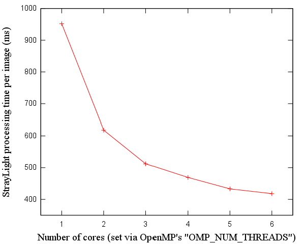
Increasing the number of threads and approaching the memory barrier
It can also be seen that the memory bandwidth is a "barrier" - as we increase the cores used, speed clearly improves less and less, in a logarithmic manner. The additional cores stress the caches more, demand more memory bandwidth, and would, eventually - if we had more than 6 cores to set OMP_NUM_THREADS to - reach a point where the performance would deteriorate instead of improve (as we saw for the SSE version of the algorithm).
4. Using a GPU (CUDA)
Modern graphics processing units (GPUs) offer massively parallel hardware architectures, allowing for optimized implementations of computational algorithms. We therefore decided to conclude our optimization efforts with an attempt to port StrayLight's convolution to the dominant GPU programming API, NVIDIA's CUDA.
4.1. Memory bandwidth and textures
We have already seen in the previous sections that whenever multithreading is put to use, there is a balancing act between the number of threads executing and the available memory bandwidth. The large number of available GPU threads (768 in the card we used [4]) makes this balancing act all the more important.
The CUDA literature points out that for algorithms that read lots of data, an efficient way to access them is to place the data inside the GPU's textures. Graphics cards' hardware has been optimized over decades to perform texture lookups in the most optimal way possible. We therefore placed the image and kernel data inside textures:
// global variables storing the two textures, that hold:

// - the input image data
texture<float1, 1, cudaReadModeElementType>     g_cudaMainMatrixTexture;

// - the convolution kernel data
texture<float1, 1, cudaReadModeElementType>     g_cudaMainKernelTexture;
...

void cudaConvolution(fp *cudaOutputImage)
{
    cudaChannelFormatDesc channel1desc = cudaCreateChannelDesc<float1>();
    cudaChannelFormatDesc channel2desc = cudaCreateChannelDesc<float1>();
    cudaBindTexture(
        NULL, &g_cudaMainMatrixTexture, cudaMainMatrix, &channel1desc,
        WIDTH*HEIGHT*sizeof(fp));
    cudaBindTexture(
        NULL, &g_cudaMainKernelTexture, cudaMainKernel, &channel2desc,
        KERNEL_SIZE*KERNEL_SIZE*sizeof(fp));
    int blks = (WIDTH*HEIGHT + THREADS_PER_BLOCK - 1)/THREADS_PER_BLOCK;
    DoWork<<< blks, THREADS_PER_BLOCK >>>(cudaOutputImage);
    // error handling
}
Note that when using double-precision, we had to resort to an official "hack" from NVIDIA's FAQ on CUDA: there are no double precision textures in CUDA, but one can emulate them via texture<int2, 1, ...>.
4.2. Running the CUDA kernel
The next step was the spawning of the CUDA convolution kernel, to be executed over hundreds of threads - more precisely, over a number of blocks, each one executing THREADS_PER_BLOCK threads. Each one of these thread blocks, is mapped by the CUDA API to a Streaming Multiprocessor (SM), and executed to completion. Each thread is computing a single output convolution "pixel".
Just as experienced for CPUs (in the previous sections), there is a "sweet spot" for the balance between the GPU's memory bandwidth and the number of threads we should actually spawn. Even though this problem is also addressed by the much faster GPU memory (GDDR5), finding the optimal balance is still necessary. To that end, we used the THREADS_PER_BLOCK macro, and fine-tuned it with testing, to make it perfectly match our own card's capacity. This was accomplished via an external Python script that automatically patched the macro definition, recompiled and benchmarked - for a range of different values of THREADS_PER_BLOCK.
Coding the actual CUDA kernel was pretty straightforward:
__global__ void DoWork(fp *cudaOutputImage)
{
    unsigned idx = blockIdx.x*blockDim.x + threadIdx.x;
    if (idx >= IMGWIDTH*IMGHEIGHT)
        return;

    // From the thread and block indexes, find the actual image sample
    // that we will be working on:
    int i = idx / IMGWIDTH;
    int j = idx % IMGWIDTH;

    // The convolution outer loops - iterating over the output image
    // 'pixels' is effected in the CUDA kernel spawning ; only the
    // convolution kernel's vertical and horizontal loops are here:
    fp sum=0.;
    for(int k=0; k<kY; k++) {
        int ofsY = i+k;
        if (ofsY>=IMGHEIGHT) ofsY -= IMGHEIGHT;

        // Compute the image and kernel lines' offsets
        // (reused in the inner loop below)
        unsigned input_image_corrected_line_Offset = IMGWIDTH*ofsY;
        unsigned psf_high_res_line_Offset = kX*k;

        #pragma unroll
        for(int l=0; l<kX; l++) {
            int ofsX = j+l;
            if (ofsX>=IMGWIDTH) ofsX -= IMGWIDTH;

            // Texture fetches - these are cached!
            sum += tex1Dfetch(g_cudaMainMatrixTexture,
                              input_image_corrected_line_Offset + ofsX).x
                   *
                   tex1Dfetch(g_cudaMainKernelTexture,
                              psf_high_res_line_Offset + l).x;
        }
    }
    int outOfsX = j+kX/2;
    if (outOfsX>=IMGWIDTH) outOfsX -= IMGWIDTH;

    int sY = i+kY/2;
    if (sY >= IMGHEIGHT) sY -= IMGHEIGHT;
    cudaOutputImage[sY*IMGWIDTH + outOfsX] = sum;
}
With the exception of using tex1Dfetch to access the 2d- image and kernel data, this code is very similar to the inner loops we wrote in the previous sections. Notice also that only the convolution-kernel-related loops are in this code, since the outer loops are hidden in the spawning of the CUDA kernel. In the beginning of the CUDA kernel, the thread and block identifiers are used to figure out which image "pixel" we will be working on in this thread.
4.3. CUDA Results
The resulting code, executed inside a relatively cheap graphics card (we used a GeForce GTX 650 Ti with 1GB GDDR5 memory, which retails at the time of writing for around 130 euros) gave a further speedup of 500% - lowering the time taken by the convolution to 51 ms, a 115x speedup (two orders of magnitude) over our initial implementation.
5. Final results and future work
We focused on the parts of the StrayLight algorithm that are executed per input image, and managed to lower them down to only 168 ms. This amounts to a 35x speedup - in the convolution, FFT, and linear interpolation stages. The previous sections demonstrated how this speedup was achieved.
There is potential for additional optimizations ; we only ported the convolution stage to CUDA, so we could simply port more. We are also paying the price for transfering the convolution input data from host to GPU memory, and transfering the output image data back out. By porting more stages of the algorithm for execution in the GPU, the transfers to and from GPU memory would be restricted to a minimum. Future work towards that direction may be necessary, if the speedup we have achieved so far is not deemed to be sufficient for the mission.
Notes
- Task 2.2 of the European Space Agency's project, "TASTE Maintenance and Evolutions" - P12001, PFL-PTE / JK / ats / 412.2012i
- REPL, Read-eval-print loop
- JIT, Just-in-Time compilation
- Development was performed on an AMD Phenom II X6 running at 3.2 GHz. The machine was equipped with 8GB of DDR3 RAM, and a GeForce GTX 650 Ti with 1GB GDDR5 memory. It was also running the stable branch of Debian Linux, with the GNU Data Language gdl interpreter installed.
- Unless frame size changes at run-time.
- To be exact: input_image_corrected is a 5271x813 float array, containing a grand total of 17MB of data (each single precision floating point number occupies 4 bytes, so 5271x813x4 = 17141292 bytes).


| Index | CV | Updated: Sat Oct 8 11:41:25 2022 |